Common Data Science Workflow

A workflow in Data Science should consist of the following steps:

1. Exploratory Data Analysis (EDA)
2. Data Cleansing
3. Model Selection
4. Model Training and Evaluation
5. Interpretation of Results

Running through those steps with the iris dataset, to which we applied random noise with a gaussian, to make this classification problem a bit harder.

# Function to add Gaussian noise
def add_gaussian_noise(data, mean=0, std=0.5):
    noise = np.random.normal(mean, std, data.shape)
    return data + noise


# Load the Iris dataset
iris = load_iris()
X = iris.data
y = iris.target

# Add noise to the features
X_noisy = add_gaussian_noise(X)

1. Exploratory Data Analysis (EDA)

The exploration starts by taken a closer look at the structure, in our case we can see statistical properties of each feature:

sepal length (cm)	sepal width (cm)	petal length (cm)	petal width (cm)	species
count	150.000000	150.000000	150.000000	150.000000	150.000000
mean	5.750400	3.066709	3.732455	1.185063	1.000000
std	0.964350	0.572030	1.852728	0.931492	0.819232
min	3.925391	1.663633	0.426725	-1.092932	0.000000
25%	5.063251	2.678627	1.666960	0.530689	0.000000
50%	5.631833	3.053473	4.298404	1.243969	1.000000
75%	6.456383	3.435793	5.097715	1.817273	2.000000
max	8.554833	4.831737	7.478399	3.107537	2.000000

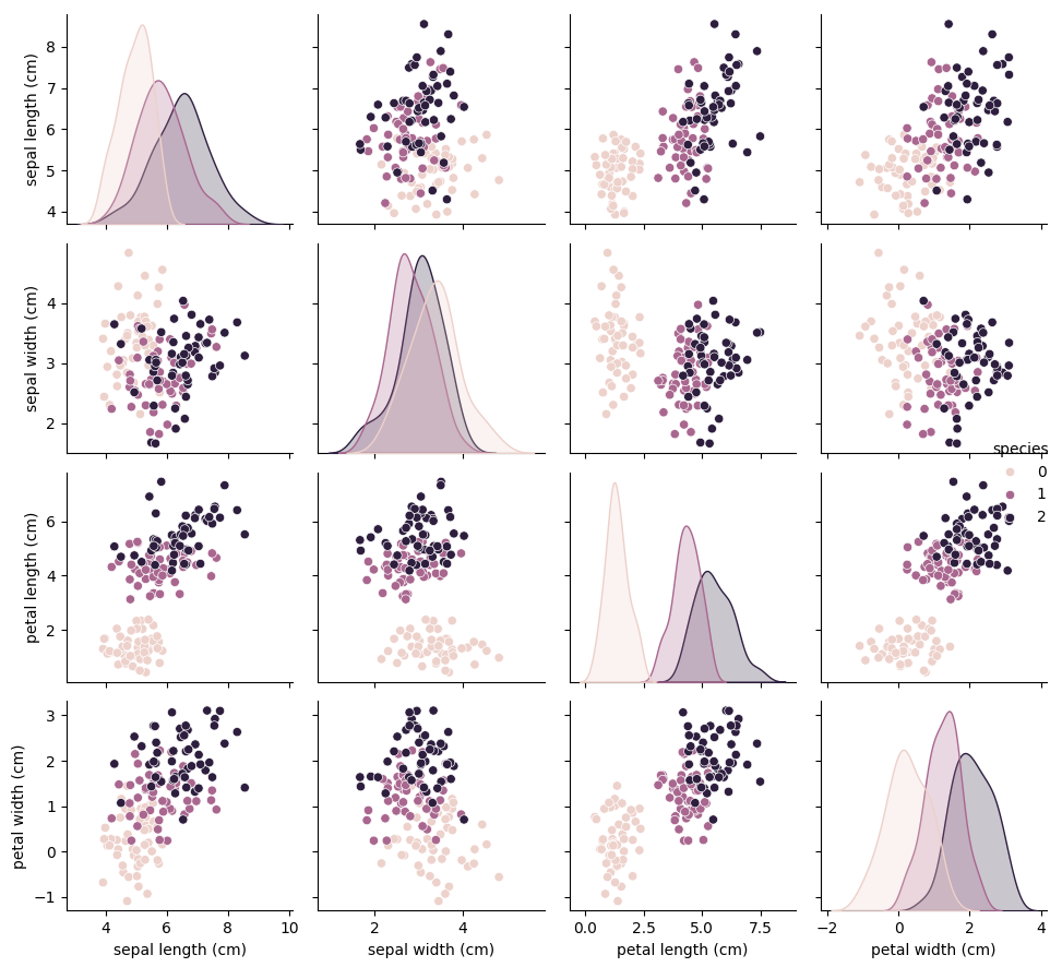
Exploring the distribution of the features is easiest with a correlation plot (the plot is created with the seaborn method pairplot). Of a given dataset each feature is plotted against all the other features, this procedure is practical to find linear correlations. Additionally, this plot shows the distribution of the features, this helps already by estimating skewness.

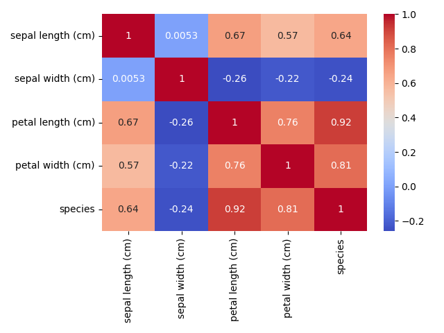
For each feature comparison in the top plot, a feature correlation coefficent can be calculated.

2. Data Cleansing

In this step, we ensure the data is clean and ready for modeling. For the Iris dataset, it is generally clean, but let’s perform a few checks, counting duplicates, dropping them, dropping rows with nan values. This is not necessarily the best pratice, how to cope with nan values depends on the problem itself, because this step may introduce a bias to your dataset.

3. Model selection

This is a classification problem. We’ll select a few models to compare. For simplicity, let’s use a Decision Tree and a Support Vector Machine (SVM).

from sklearn.model_selection import train_test_split
from sklearn.tree import DecisionTreeClassifier
from sklearn.svm import SVC

# Split the data into training and testing sets
X = df.drop("species", axis=1)
y = df["species"]
X_train, X_test, y_train, y_test = train_test_split(
    X, y, test_size=0.5, random_state=42
)

# Initialize the models
dt_model = DecisionTreeClassifier()
svm_model = SVC()

# Train the models
dt_model.fit(X_train, y_train)
svm_model.fit(X_train, y_train)

4. Model Training and Evaluation

We’ll evaluate the models using accuracy scores and confusion matrices. \(\text{Decision Tree Accuracy: } 0.86\) \(\text{SVM Accuracy: } 0.92\) Understand the true positives, true negatives, false positives, and false negatives for each model. We already see that there are fewer false positive detections by SVM. \(\text{Decision Tree Confusion Matrix} = \begin{bmatrix} 29 & 0 & 0 \\\ 0 &20 & 3\\\ 0 & 7 &16\end{bmatrix}\) \(\text{SVM Confusion Matrix} = \begin{bmatrix} 29 & 0 & 0 \\\ 0 &20 & 3\\\ 0 & 3 &20\end{bmatrix}\)

The classification report provides a detailed performance evaluation of the model by presenting precision, recall, and F1-score for each class, allowing us to understand how well the model distinguishes between different categories. Precision measures the accuracy of positive predictions, recall indicates the model’s ability to find all relevant instances, and F1-score provides a balance between precision and recall, offering a comprehensive view of model performance.

Decision Tree Classification Report:

-	precision	recall	f1-score	support
0	1.00	1.00	1.00	29
1	0.74	0.87	0.80	23
2	0.84	0.70	0.76	23
accuracy	-	-	0.87	75
macro avg	0.86	0.86	0.85	75
weighted avg	0.87	0.87	0.87	75

SVM Classification Report:

-	precision	recall	f1-score	support
0	1.00	1.00	1.00	29
1	0.87	0.87	0.87	23
2	0.87	0.87	0.87	23
accuracy	-	-	0.92	75
macro avg	0.91	0.91	0.91	75
weighted avg	0.92	0.92	0.92	75

Based on the classification report SVM classification is superior to the Decision Tree Classifictaion.